NEURON + Python Basics
The objectives of this part of the tutorial are to get familiar with basic operations of NEURON using Python. In this worksheet we will:
- Create a passive cell membrane in NEURON.
- Create a synaptic stimulus onto the neuron.
- Modify parameters of the membrane and stimulus.
- Visualize results with matplotlib.
What is NEURON?
The NEURON simulation environment is a powerful engine for performing simulations of neurons and biophysical neural networks. It permits the construction of biologically realistic membranes with active and passive ion channels, combined with virtual connectivity and electrophysiology tools to drive and measure neuron and network behaviors.
Step 1: Import the neuron module into Python.
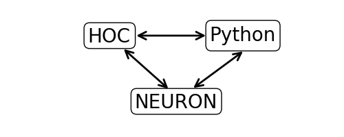
Any code that is not part of Python’s Built-in Functions must be imported. The Python interface to NEURON goes through the “h” module. The h module permits a direct interface to NEURON as well as to NEURON’s other interpreter language, hoc. This permits Python to utilize existing hoc models (or parts of models). The relationships of these modules are illustrated below.
We begin by loading NEURON’s h module and its graphical user interface:
from neuron import h, gui
The results of evaluating this code should look something like the following output.
NEURON -- VERSION 7.5 master (6b4c19f) 2017-09-25
Duke, Yale, and the BlueBrain Project -- Copyright 1984-2016
See http://neuron.yale.edu/neuron/credits
Step 2: Create a cell
We create a simple model cell as a NEURON Section. Evaluate the line below:
soma = h.Section(name='soma')
There is no output, so how can we tell we successfully created a section?
Aside 1: NEURON’s psection() function.
NEURON’s psection() (short for “print section”) function can provide a lot of detail on sections. Let’s validate that we have a soma and view some of its properties.
h.psection()
The results tell us the soma is a cylinder with length 100 microns, diameter 500 microns, axial resistivity 35.4 ohm*cm, and specific membrance capacitance 1 \(\mu F/cm^2\)
Aside 2: Python’s dir() function.
We can also probe objects with Python’s built-in dir() function. Let’s see what it says about soma.
dir(soma)
This tells us all of the Python methods and variables associated with the object. Any methods with two leading and trailing underscores are reserved by Python and may or may not be implemented by the object. The other items in the list are additional members of soma that we can call. To see all of the functions available to the neuron variable h, try calling dir(h).
Biophysical Mechanisms
NEURON comes with a few built in biophysical mechanisms that can be added to a model.
pas |
Passive (“leak”) channel. |
extracellular |
For simulating effects of nonzero extracellular potential, as may happen with leaky patch clamps, or detailed propertes of the myelin sheath. |
hh |
Hodgkin-Huxley sodium, potassium, and leakage channels. |
Step 3: Insert a passive mechanism.
We see from the list of elements after calling dir(soma) that insert is available. This is the method we will use to insert mechanisms into the membrane. Let’s insert a passive leak conductance across the membrane and do this by passing ‘pas’ as the mechanism type:
soma.insert('pas')
Aside 4: Sections and segments.
A NEURON Section is considered a piece of cylindrical cable. Depending on the resolution desired, it may be necessary to divide the cable into a number of segments where voltage varies linearly between centers of adjacent segments. The number of segments within a section is given by the variable, nseg. The total ionic current across the segment membrane is approximately the area of the segment multiplied by the ionic current density at the center of the segment. To access a part of the section, specify a value between 0 and 1, where 0 is typically the end closest to the soma and 1 is the distal end. Because nseg divides the cable into equal-length parts, it should be an odd number so that to address the middle of the cable, (0.5), gives the middle segment.
To summarize, we access sections by their name and segments by some location on the section.
- Section:
section - Segment:
section(loc)
Using the Python type() function can tell us what a variable is:
print("type(soma) = {}".format(type(soma)))
print("type(soma(0.5)) ={}".format(type(soma(0.5))))
Aside 5: Accessing segment variables.
Segment variables follow the idiom:
section(loc).var
And for mechanisms on the segment:
section(loc).mech.var
or
section(loc).var_mech
The first form is preferred.
mech = soma(0.5).pas
print(dir(mech))
print(mech.g)
print(soma(0.5).pas.g)
Step 4: Insert an alpha synapse.
Let’s insert an AlphaSynapse object onto the soma to induce some membrane dynamics.
asyn = h.AlphaSynapse(soma(0.5))
AlphaSynapse is a Point Process. Point processes are point sources of current. When making a new PointProcess, you pass the segment to which it will bind.
Again, with dir() function, we can validate that asyn is an object and contains some useful parameters. Let’s look at some of those parameters.
dir(asyn)
print("asyn.e = {}".format(asyn.e))
print("asyn.gmax = {}".format(asyn.gmax))
print("asyn.onset = {}".format(asyn.onset))
print("asyn.tau = {}".format(asyn.tau))
Let’s assign the onset of this synapse to occur at 20 ms and the maximal conductance to 1.
asyn.onset = 20
asyn.gmax = 1
Let’s look at the state of our cell using neuron’s psection().
h.psection()
Step 5: Set up recording variables.
The cell should be configured to run a simulation. However, we need to set up variables we wish to record from the simulation. For now, we will record the membrane potential, which is soma(0.5).v. References to variables are available as _ref_rangevariable.
v_vec = h.Vector()             # Membrane potential vector
t_vec = h.Vector()             # Time stamp vector
v_vec.record(soma(0.5)._ref_v)
t_vec.record(h._ref_t)
Step 6: Run the simulation.
To run the simulation, we execute the following lines.
h.tstop = 40.0
h.run()
Note
If we had not included gui in the list of things to import, we would
have also had to execute:
h.load_file('stdrun.hoc')
which defines the run() function (the alternative would be to specify
initialization and advance in more detail).
Step 7: Plot the results.
We utilize the pyplot module from the matplotlib Python package to visualize the output.
from matplotlib import pyplot
pyplot.figure(figsize=(8,4)) # Default figsize is (8,6)
pyplot.plot(t_vec, v_vec)
pyplot.xlabel('time (ms)')
pyplot.ylabel('mV')
pyplot.show()
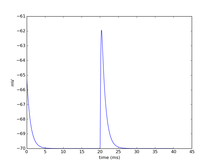
The last line displays the graph and allows you to interact with it (zoom, pan, save, etc). NEURON and Python will wait until you close the figure window to proceed.
Step 8: Saving and restoring results.
NEURON Vector objects can be pickled. This allows them to be stored to disk and restored later:
Saving:
# Pickle
import pickle
with open('t_vec.p', 'wb') as t_vec_file:
    pickle.dump(t_vec, t_vec_file)
with open('v_vec.p', 'wb') as v_vec_file:
    pickle.dump(v_vec, v_vec_file)
Loading:
from neuron import h, gui
from matplotlib import pyplot
import pickle

# Unpickle
with open('t_vec.p', 'rb') as t_vec_file:
    t_vec = pickle.load(t_vec_file)
with open('v_vec.p', 'rb') as vec_file:
    v_vec = pickle.load(vec_file)

# Confirm
pyplot.figure(figsize=(8,4)) # Default figsize is (8,6)
pyplot.plot(t_vec, v_vec)
pyplot.xlabel('time (ms)')
pyplot.ylabel('mV')
pyplot.show()