Ball-and-stick: 1 - Basic cell¶

A newer version of this tutorial is available

This is the first of several pages to build a multicompartment cell and evolve it into a network of cells running on a parallel machine. While design of the model and its underlying code are paramount for maintenance and extending the project, realizing such designs tend to occur as needed. These tutorials therefore take a functional approach by adding in design as the project gets more complex rather than describing a complex design and filling in the pieces.

This page builds a two-compartment cell, a soma and dendrite, which is simply known as a ball-and-stick model. After building the cell we will to attach some instrumentation to it to stimulate and monitor its dynamics.

Cell model design¶

When building a biophysical cell, it is best to segregate the construction into parts. This facilitates clarity and stepwise development. It also makes debugging, extending, and translating to parallel implementations much easier.

The parts of the cell model are:

Sections - the cell sections.
Topology - The connectivity of the sections
Geometry - The 3D location of the sections
Biophysics - The ionic channels and membrane properties of the sections
Synapses - Optional list of synapses onto the cell.

Ball-and-stick model¶

We will start with a ball-and-stick model, a soma connected to a dendrite.

Start by importing NEURON.

from neuron import h, gui

Create our sections¶

soma = h.Section(name='soma')
dend = h.Section(name='dend')

Remember h.psection to retrieve information. Note that when there is more than one section, we need to pass in a section to specify which one we want to see informatin about:

h.psection(sec=soma)

Topology¶

Connect the dendrite to the “1” end of the soma.

dend.connect(soma(1))

Let’s check the connection.

h.psection(sec=dend)

Let’s further confirm with NEURON’s topology() function.

h.topology()

Both of these approaches show that dend[0] is connected to soma[1].

Geometry¶

Let’s set the spatial properties of the cell using a “stylized” geometry. Later we will explore setting 3D points explicitly.

# Surface area of cylinder is 2*pi*r*h (sealed ends are implicit).
# Here we make a square cylinder in that the diameter
# is equal to the height, so diam = h. ==> Area = 4*pi*r^2
# We want a soma of 500 microns squared:
# r^2 = 500/(4*pi) ==> r = 6.2078, diam = 12.6157
soma.L = soma.diam = 12.6157 # Makes a soma of 500 microns squared.
dend.L = 200 # microns
dend.diam = 1 # microns
print("Surface area of soma = {}".format(soma(0.5).area()))

Now we can see what our cell looks like. From the GUI, we can select Graph ‣ Shape plot or we can run the following command:

shape_window = h.PlotShape()

The image might not be what you expect at first:

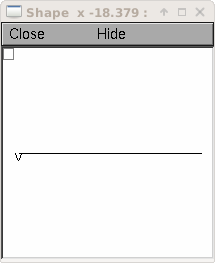
What happened? It looks like a line because there are only two sections and NEURON by default does not display diameters. This behavior is useful when we need to see the structure of small dendrites, but for now let’s show the diameters. We do this by either right-clicking on the graph and selecting Shape Style ‣ Show Diam (in lieu of right clicking, we can left-click on the box in the upper left of the graph) or by running the following command:

shape_window.exec_menu('Show Diam')

Either way, we now see the “ball-and-stick” morphology, where the soma is a relatively large ball attached to a long stick-like dendrite:

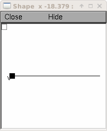
We can rotate the image by right-clicking and selecting 3D Rotate, but for this simple of a morphology, there is not anything more to see.

Note

Matplotlib and Mayavi can also be used to generate 3D pictures of neurons. To use this, use h.allsec() to iterate over all the sections, read their 3D points, and use those to define their geometries.

Biophysics¶

Our cell needs biophysical mechanisms in the membrane.

for sec in h.allsec():
    sec.Ra = 100    # Axial resistance in Ohm * cm
    sec.cm = 1      # Membrane capacitance in micro Farads / cm^2

# Insert active Hodgkin-Huxley current in the soma
soma.insert('hh')
for seg in soma:
    seg.hh.gnabar = 0.12  # Sodium conductance in S/cm2
    seg.hh.gkbar = 0.036  # Potassium conductance in S/cm2
    seg.hh.gl = 0.0003    # Leak conductance in S/cm2
    seg.hh.el = -54.3     # Reversal potential in mV

# Insert passive current in the dendrite
dend.insert('pas')
for seg in dend:
    seg.pas.g = 0.001  # Passive conductance in S/cm2
    seg.pas.e = -65    # Leak reversal potential mV

If you want to know the units for a given mechanism’s parameter, use units(). Pass in a string with the paramater name, an underscore, and then the mechanism name.

print(h.units('gnabar_hh'))

Confirm with psection().

for sec in h.allsec():
    h.psection(sec=sec)

Note

Technically, we do not need to specify the section with a sec= keyword argument to psection() here because when iterating over h.allsec() the current section becomes NEURON’s default section, but it’s best practice to never depend on the default section.

Instrumentation¶

We have now created our cell. Let’s stimulate it and visualize its dynamics.

Stimulation¶

Let’s inject a current pulse into the distal end of the dendrite. We will give it the properties of starting 5 ms after the simulation starts, with a duration of 1 ms, and with an amperage of 0.1 nA.

stim = h.IClamp(dend(1))

Let’s see the attributes of stim.

dir(stim)

So let’s verify the location.

print("segment = {}".format(stim.get_segment()))

Let’s set our fields.

stim.delay = 5
stim.dur = 1
stim.amp = 0.1

Set up the recording vectors, run, and plot.

v_vec = h.Vector()        # Membrane potential vector
t_vec = h.Vector()        # Time stamp vector
v_vec.record(soma(0.5)._ref_v)
t_vec.record(h._ref_t)
simdur = 25.0

h.tstop = simdur
h.run()

from matplotlib import pyplot
pyplot.figure(figsize=(8,4)) # Default figsize is (8,6)
pyplot.plot(t_vec, v_vec)
pyplot.xlabel('time (ms)')
pyplot.ylabel('mV')
pyplot.show()

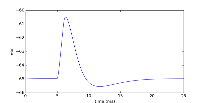
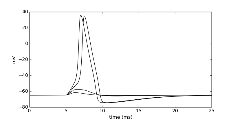
It looks like we have a dynamic cell. Let’s push it a little. Let’s vary the amplitude of the current in a loop.

import numpy
pyplot.figure(figsize=(8,4))
step = 0.075
num_steps = 4
for i in numpy.linspace(step, step*num_steps, num_steps):
    stim.amp = i
    h.tstop = simdur
    h.run()
    pyplot.plot(t_vec, v_vec, color='black')

pyplot.xlabel('time (ms)')
pyplot.ylabel('mV')
pyplot.show()

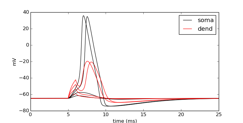
Let’s also visualize what is going on in the dendrite. Notice that we do not have to re-assign the time and soma membrane potential recording vectors, but we make a new one in the middle of the dendrite.

dend_v_vec = h.Vector()        # Membrane potential vector
dend_v_vec.record(dend(0.5)._ref_v)

pyplot.figure(figsize=(8,4))
for i in numpy.linspace(step, step*num_steps, num_steps):
    stim.amp = i
    h.tstop = simdur
    h.run()
    soma_plot = pyplot.plot(t_vec, v_vec, color='black')
    dend_plot = pyplot.plot(t_vec, dend_v_vec, color='red')

# After looping, actually draw the image with show.
# For legend labels, use the last instances we plotted
pyplot.legend(soma_plot + dend_plot, ['soma', 'dend'])
pyplot.xlabel('time (ms)')
pyplot.ylabel('mV')
pyplot.show()

Let’s push it a bit more. Let’s see the effects of nseg, the number of segments of the dendrite, on the signal through the dendrite.

To do the comparison, let’s start by rerunning without displaying the plot:

pyplot.figure(figsize=(8,4))
for i in numpy.linspace(step, step*num_steps, num_steps):
    stim.amp = i
    h.run()
    soma_plot = pyplot.plot(t_vec, v_vec, color='black')
    dend_plot = pyplot.plot(t_vec, dend_v_vec, color='red')

We will now increase the number of segments in the dendrite from 1 (the default) to 101:

dend.nseg = 101

and then plot the same simulations, this time displaying everything when we’re done:

for i in numpy.linspace(step, step*num_steps, num_steps):
    stim.amp = i
    h.run()
    soma_hires = pyplot.plot(t_vec, v_vec, color='blue')
    dend_hires = pyplot.plot(t_vec, dend_v_vec, color='green')

# After looping, actually draw the image with show.
# For legend labels, use the last instances we plotted
pyplot.legend(soma_plot + dend_plot + soma_hires + dend_hires, ['soma', 'dend', 'soma hi-res', 'dend hi-res'])
pyplot.xlabel('time (ms)')
pyplot.ylabel('mV')
pyplot.show()

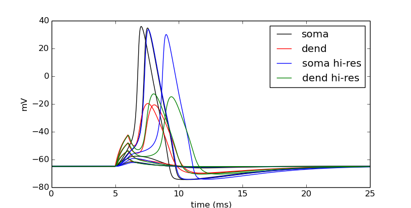
We can tell in this case, that having a large number of segments in the dendritic section modifies the output. The blue and green are high resolution output. We would like to determine a minimal number of segments that still give largely accurate results.

Let’s modify nseg to other values. What values overlay the blue and green lines well? (Remember, since we are showing results at 0.5 in the dendrite, nseg should be an odd value). Let’s also quantify the error by subtracting the vectors between the high-resolution output with the result with a particular value of nseg.

pyplot.figure(figsize=(8,4))
ref_v = []
ref_dend_v = []

# Run through the cases of high resolution
dend.nseg = 101
for i in numpy.linspace(step, step*num_steps, num_steps):
    stim.amp = i
    h.run()
    soma_hires = pyplot.plot(t_vec, v_vec, color='blue')
    soma_hires = pyplot.plot(t_vec, dend_v_vec, color='green')
    # Copy the values of these "reference" vectors for use below
    ref_v_vec = numpy.zeros_like(v_vec)
    v_vec.to_python(ref_v_vec)
    ref_v.append(ref_v_vec)
    ref_dend_v_vec = numpy.zeros_like(dend_v_vec)
    dend_v_vec.to_python(ref_dend_v_vec)
    ref_dend_v.append(ref_dend_v_vec)

# Run through the cases of lower resolution
dend.nseg = 1 #### Play with this value. Use odd values. ####

err = 0
idx = 0
for i in numpy.arange(step, step*(num_steps+.9), step):
    stim.amp = i
    h.run()
    soma_lowres = pyplot.plot(t_vec, v_vec, color='black')
    dend_lowres = pyplot.plot(t_vec, dend_v_vec, color='red')
    err += numpy.mean(numpy.abs(numpy.subtract(ref_v[idx], v_vec)))
    err += numpy.mean(numpy.abs(numpy.subtract(ref_dend_v[idx], dend_v_vec)))
    idx += 1

err /= idx
err /= 2 # Since we have a soma and dend vec

print("Average error = {}".format(err))

pyplot.legend(soma_lowres + dend_lowres + soma_hires + dend_hires,
        ['soma low-res', 'dend low-res', 'soma hi-res', 'dend hi-res'])
pyplot.xlabel('time (ms)')
pyplot.ylabel('mV')
pyplot.show()

The figure is the same as before except for the legend.

By replacing the dend.nseg = 1 value with higher odd numbers and rerunning we can see both graphically and quantitatively how the results depend on nseg. With dend.nseg = 1, the error is 2.61016682451; with dend.nseg = 11, the error drops to 0.065745004413.

Ball-and-stick: 1 - Basic cell¶

Cell model design¶

Ball-and-stick model¶

Create our sections¶

Topology¶

Geometry¶

Biophysics¶

Instrumentation¶

Stimulation¶

Table Of Contents

Previous topic

Next topic

This Page