Reaction-Diffusion
Overview
Concept
Proteins, ions, etc... in a cell perform signalling functions by moving, reacting with other molecules, or both. In some cases, this movement is by active transport processes, which we do not consider here. If all movement is due to diffusion (wherein a molecule moves randomly), then such systems are known as reaction-diffusion systems.
These problems are characterized by the answers to three questions: (1) Where do the dynamics occur, (2) Who are the actors, and (3) How do they interact?
Math
Reaction-diffusion equations are equations or systems of equations of the form
where \(u\) is the concentration of some state variable and \(\nabla^2\) is the Laplacian operator. In one-dimensional Cartesian space, \(\nabla^2 u = u_{xx}\), while in three-dimensional Cartesian space \(\nabla^2 u = u_{xx} + u_{yy} + u_{zz}\). This form follows from Fick’s law of diffusion and the Divergence theorem and assumes that the diffusion constant \(d\) is uniform throughout the spatial domain.
Note
Can also have systems of equations. If \(d\) is nonuniform, it goes inside one of the \(\nabla\)s.
Specification
To describe a reaction-diffusion problem in NEURON, begin by loading the rxd library:
from neuron import rxd
Then answer the three questions: where, who, and how.
Where
We begin by identifying the domain; i.e. where do the dynamics occur? For many electrophysiology simulations, the only relevant domains are the plasma membrane or the volumes immediately adjacent to it on either side, since these are the regions responsible for generating the action potential. Cell biology models, by contrast, have dynamics spanning a more varied set of locations. In addition to the previous three regions, the endoplasmic reticulum (ER), mitochondria, and nuclear envelop often play key roles.
The rxd.Region class is used to describe the domain:
r = rxd.Region(sections, nrn_region=None, geometry=None)
In its simplest usage, rxd.Region simply takes a Python iterable (e.g. a list or a nrn.SectionList) of nrn.Section objects. In this case, the domain is the interior of the sections, but the concentrations for any species created on such a domain will only be available through the rxd.Species object and not through HOC or NMODL.
Example: Region on all sections:
r = rxd.Region(h.allsec())
Example: Region on just a few sections:
r = rxd.Region([soma, apical1, apical2])
If the region you are describing coincides with the domain on the immediate interior of the membrane, set nrn_region='i', e.g.
r = rxd.Region(h.allsec(), nrn_region='i')
Concentration in these regions increases when a molecule of the species of interest crosses from outside the membrane to the inside via an NMODL or kschan mechanism. If a species on such a region is named ca, then its concentrations can be read and set via the HOC and NMODL range variable cai.
Also: outside the membrane with nrn_region='o'
Many alternative geometries, including: rxd.membrane, rxd.inside, rxd.Shell, rxd.FractionalVolume, rxd.FixedCrossSection, rxd.FixedPerimeter.
Who
Who are the actors? Often they are chemical species (proteins, ions), sometimes they are State variables (such as a gating variable), and other times parameters that vary throughout the domain are key actors. All three of these can be described using the rxd.Species class:
s = rxd.Species(regions=None, d=0, name=None, charge=0, initial=None)
although we also provide rxd.State and rxd.Parameter for the second and third case, respectively. For now these are exact synonyms of rxd.Species that exist for promoting the clarity of the model code, but this will likely change in the future (so that States can only be changed over time via Rate objects and that Parameters will no longer occupy space in the integration matrix.)
Note
charge must match the charges specified in NMODL files for the same ion, if any.
The regions parameter is mandatory and is either a single rxd.Region or an iterable of them, and specifies what region(s) contain the species.
Set d= to the diffusion constant for your species, if any.
Specify an option for the name= keyword argument to allow these state variables to map to the HOC/NMODL range variables if the regions nrn_region is i or o.
Specify initial conditions via the initial= keyword argument. Set that to either a constant or a function that takes a node (see below).
Example: to have concentrations set to 47 at finitialize():
s = rxd.Species(region, initial=47)
Warning
For consistency with the rest of NEURON, the units of concentration are assumed to be in mM. Many cell biology models involve concentrations on the order of μM.
Warning
There is currently a bug in initial support: if initial=None and name=None, then concentration will not be changed at a subsequent finitialize(). The intended behavior is that this would reset the concentration to 0.
initial is also a property of the Species/Parameter/State s and may be changed at any time, as in:
s.initial = 3.14159
How
How do they interact? Species interact via one or more chemical reactions. The primary class used to specify reactions is rxd.Reaction:
r = rxd.Reaction(scheme, rate_f, rate_b=None, regions=None, custom_dynamics=False)
Here scheme is a reaction scheme, which indicates that the reaction takes one arithmetic sum of integer multiples of molecules to another. For example, a scheme for an irreversible reaction to form table salt might be Na + Cl > NaCl. The forward arrow > indicates that the reaction is irreversible and only proceeds from left-to-right. A reverse arrow < indicates an irreversible reaction that only proceeds from right-to-left. Most reactions are to at least some extent bidirectional, which we indicate using the bidirectional arrow <>.
Once we have specify which molecules get transformed into what, it remains to specify how quickly these reactions occur.
(Reaction, but also Rate and MultiCompartmentReaction)
Contrast Reaction and Rate... use Rate for arbitrary changes to one species... e.g. non-oc
Example: Water bonding (mass action)
r = rxd.Reaction(2 * hydrogen + oxygen > water, k1)
This translates into the system of differential equations:
\[\begin{split}h' &= - 2\, k_1 \, h ^ 2 \, o \\ o' &= - k_1 \, h ^ 2 \, o \\ w' &= k_1 \, h ^ 2 \, o\end{split}\]
Warning
The reaction scheme is interpreted as a statement about a single molecular reaction. That is, if the scheme involves \(aA + bB + cC\), then \(a\), \(b\), and \(c\) are the stoichiometry coefficients.
In particular, this means the reaction 2 * hydrogen + oxygen > water is not equivalent to 4 * hydrogen + 2 * oxygen > 2 * water as the second requires four hydrogen molecules and two oxygen molecules to come together simultaneously before any reaction occurs (which causes the \(h\) to be raised to the fourth power in the differential equations instead of to the second power).
For more background, see the Wikipedia article on the rate equation.
Reactions conserve mass. This property is especially important for stochastic simulations. Often, however, one might wish to model a source or a sink, or describe the dynamics of a state variable that is not a concentration. In this case, use the non-conservative rxd.Rate.
r = rxd.Rate(var, react_rate, regions=None)
This line only changes the Species/State variable var and it does so by adding react_rate to the right hand side of the equation. For example, assuming h and rxd have been defined in the usual way, then
all = rxd.Region(h.allsec())
u = rxd.Species(all, d=1, initial=0)
bistable_reaction = rxd.Rate(u, -u * (1 - u) * (0.3 - u))
is equivalent to the equation
This example is explored in more detail in Scalar Bistable Wave.
As with rxd.Reaction, if regions is ommitted or None, then the dynamics specified here will occur on every region containing var and every variable mentioned in rate. If, instead, regions is a Python iterable, then the dynamics will be further restricted to those regions also listed in the iterable.
Reading the Data
NodeList
For a given species s, s.nodes is a NodeList of all of its nodes. NodeList objects are derived from the Python list, so they offer all the same methods, e.g. one can access the first node
node = s.nodes[0]
or get the total number of nodes
num_nodes = len(s.nodes)
exactly as if s.nodes was a list, but one can also read and set concentrations (concentration) and diffusion constants (diff) for all nodes in the NodeList in a vectorized way, as well as read the volumes (volume), surface areas (surface_area), regions (region), species (species), and normalized positions (x). For example, to get lists of positions (x) and concentrations (y) suitable for plotting from the NodeList nl, use
x = nl.x
y = nl.concentration
When assigning concentration or the diffusion constant, one can either set them equal to an iterable with the same length as the NodeList or to a scalar as in
nl.concentration = 47
Calling a NodeList returns a sub-NodeList of nodes satisfying a given restriction. For example,
nl(soma)
returns a NodeList of all Nodes lying in the nrn.Section named “soma.” As this is itself a NodeList, we can get a list of the nodes from nl in the soma section belonging to the rxd.Region “er”:
nl(soma)(er)
Valid restrictions for now are section objects, region objects, and normalized position 0 <= x <= 1. Restrictions are implemented via the satisfies method of individual nodes. If you would like to extend the set of restrictions, either send me a patch or at least make a specific proposal.
Warning
The experimental 3d support currently uses lists instead of NodeLists, but it could be easily switched to use NodeLists.
Node
Sometimes though, it is important to work with an individual Node, such as for communication with nmodl or for plotting. The Graph.addvar() method, for example, needs a HOC reference to the memory location containing the concentration, which is available via the _ref_concentration property:
g.addvar('calcium', node._ref_concentration)
If a node is mapped to a HOC range variable (that is, if the species name is specified and the Region’s nrn_region is i or o), then there are three equivalent ways to read/set the concentration in 1d simulations. Here we assume the species is named ca and the nrn_region=`i` and that the node is at 0.5 in the currently accessed section:
h.cai(0.5) = 1.618
node.concentration = 1.618
node._ref_concentration[0] = 1.618
Warning
In 1d, all three will always report the same value. In 3d, however, the values in the HOC range variables are averaged values, and changing those will not change the 3d values.
All the properties of NodeList are also available in individual Nodes, with the exception that all values are scalars and not vectors.
Examples
Simple Reaction with Abrupt Change in Reaction Rate
from neuron import h, rxd

dend = h.Section()
r = rxd.Region(h.allsec())

hydrogen = rxd.Species(r, initial=1)
oxygen = rxd.Species(r, initial=1)
water = rxd.Species(r, initial=0)

reaction = rxd.Reaction(2 * hydrogen + oxygen > water, 1)

h.finitialize()

heading = '{t:>10s}  {h:>10s}  {o:>10s}  {h2o:>10s}'
data = '{t:10g}  {h:10g}  {o:10g}  {h2o:10g}'

def advance_a_bit():
    for i in xrange(5):
        h.fadvance()
        print data.format(t=h.t, h=hydrogen.nodes[0].concentration,
                          o=oxygen.nodes[0].concentration,
                          h2o=water.nodes[0].concentration)

print heading.format(t='t', h='hydrogen', o='oxygen', h2o='H2O')
print heading.format(t='-', h='--------', o='------', h2o='---')

advance_a_bit()

# increase the forward reaction rate
reaction.f_rate *= 5

print
print '---- water production rate should speed up below here ----'
print

advance_a_bit()
Output:
         t    hydrogen      oxygen         H2O
         -    --------      ------         ---
     0.025    0.955556    0.977778   0.0222222
      0.05    0.915565    0.957783   0.0422175
     0.075    0.879356    0.939678   0.0603222
       0.1    0.846386    0.923193   0.0768069
     0.125    0.816217    0.908108   0.0918917

---- water production rate should speed up below here ----

      0.15    0.712186    0.856093    0.143907
     0.175    0.632848    0.816424    0.183576
       0.2    0.570372    0.785186    0.214814
     0.225    0.519873    0.759937    0.240063
      0.25    0.478173    0.739086    0.260914
Diffusion and Interaction with Ion Channels
(This is analogous to the old nadifl1 example)
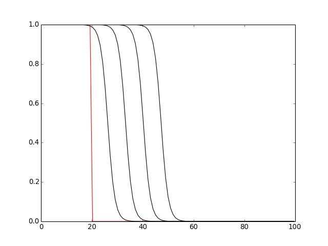
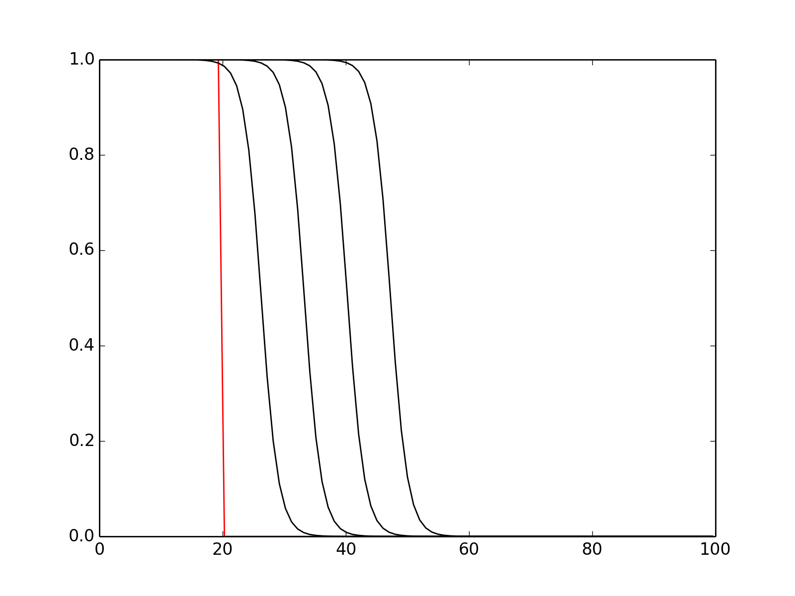
Scalar Bistable Wave
This is a specific propagating wave. A classic test because the exact analytic solution is known on the real line.
from neuron import h, rxd
import numpy
from matplotlib import pyplot

# needed for standard run system
h.load_file('stdrun.hoc')

dend = h.Section()
dend.nseg = 101

# WHERE the dynamics will take place
where = rxd.Region(h.allsec())

# WHO the actors are
u = rxd.Species(where, d=1, initial=0)

# HOW they act
bistable_reaction = rxd.Rate(u, -u * (1 - u) * (0.3 - u))

# initial conditions
h.finitialize()
for node in u.nodes:
    if node.x < .2: node.concentration = 1

def plot_it(color='k'):
    y = u.nodes.concentration
    x = u.nodes.x

    # convert x from normalized position to microns
    x = dend.L * numpy.array(x)

    pyplot.plot(x, y, color)

plot_it('r')

for i in xrange(1, 5):
    h.continuerun(i * 25)
    plot_it()

pyplot.show()
(Source code, png, hires.png, pdf)