Step 6. Perform the optimization

A. Test the MRF

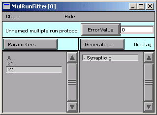
We click on the MRF's Error Value button and . . . nothing happens.
The value displayed in the adjacent field is still 0.

Ah--we haven't told the MRF to use our Synaptic g generator.
See the little - (minus) sign in front of the generator's name?

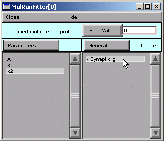
So we click on Generators / Use Generator

Notice the "Toggle" next to the Generators button.
Double clicking on "Synaptic g" in the MRF's right panel turns this generator on. If we double click on it again, it will turn back off--no big deal, because we can always turn it back on again.

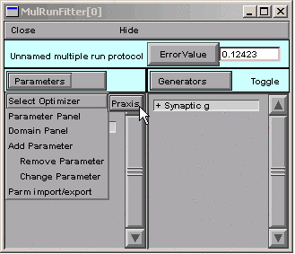
The + signifies that the Synaptic g generator is on. This means that, when we click on the Error Value button in the MRF, the Synaptic g generator will be used and will contribute to the total error value that appears in the adjacent numeric field.

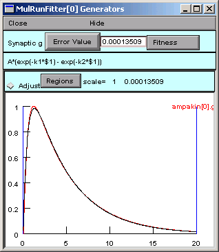
So we click on the MRF's Error Value button, and we see a nonzero value in the Error Value field. This confirms that we're using the Synaptic g generator.

Is this is a good time to save to a session file, or what?

B. Choose and use an optimization algorithm

At last, we're ready to choose an optimization algorithm and use it. The only one currently available is Praxis.
Parameters / Select Optimizers / Praxis

Selecting the Praxis optimizer brings up a MulRunFitter Optimize window (we'll just call this the "Optimize window").

Now we click on the Optimize button in the Optimize window.

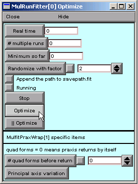
Several iterations flash by in the Generator, and we soon see the result of optimization.

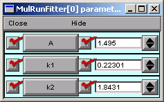
To examine the parameter values the optimizer settled on, we need to look at a Parameter panel.
Hint : in the MRF, click on Parameters / Parameter Panel

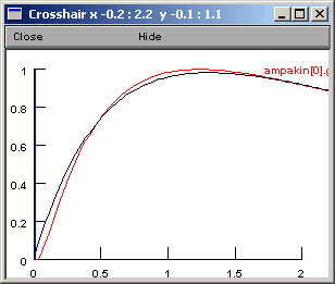
The fit looks nice, but the peak isn't quite perfect. Closer examination (New view in Generator) shows that the double exponential function starts to rise immediately, unlike the experimental data, which show an initial lag in the rise of synaptic condctance (sigmoidal onset).

Whether this discrepancy matters or not depends entirely on what we intend to do with the optimized function.

If you really have to know why there is an initial delay in the rising phase of g, the answer is that, although transmitter release is "instantaneous," channel opening requires two reactions with finite rates (binding of transmitter A to the closed Rc, and conversion of the closed ARc to the open ARo).

"Extra credit" problem

1. Note the final parameter values and the Error Value.
2. Restore the parameters to their initial values (A = 1, k1 = 1, k2 = 10),
   specify linear scaling, and try another optimization.
   Was optimization any faster?
   What difference did this make in the optimized parameters and Error Value?

   It turns out that log scaling is not critical for the present example,
   because the optimum parameter values span only one order of magnitude.

   Now see what happens when the parameters have very different magnitudes.

3. Read the data file into NEURON's clipboard, and then type
      hoc_obj_[0].mul(1e-5)
   at the oc> prompt. This makes the data values 5 orders of magnitude smaller.
4. Transfer these scaled data into the Generator (Regions / Data from Clipboard).
5. In the Parameter Panel, set k1 = 1, k2 = 10, and A = 1e-5.
6. In the Domain Panel, go back to linear scaling.
7. Click on the Error Value button (either in the Generator or in the MRF).
   Notice that the black and red traces have exactly the same shapes as when we used the unscaled data.
8. Now click on the Optimize button.
   Watch what happens as the optimizer tries to fit the data.
   Are things going as smoothly as with the unscaled data?
   Optimize again, and again, if you have to.
   What do you think about the speed of convergence and the quality of the fit?
9. Restore the parameters to k1 = 1, k2 = 10, and A = 1e-5,
   specify log scaling, and try another optimization.

   Did log scaling help when the optimum parameter values had very different magnitudes?

Hints

Local minima

Poor fits may result if the optimizer falls into a local minimum of the objective function. To check for this possibility, bounce it out of there by clicking on the "Randomize with factor" button, and then start another optimization. You may want to increase the randomization factor from its default value of 2.

Adjustable parameters

In the Parameter Panel (MRF / Parameters / Parameter Panel) you may have noticed the checkboxes to the left of the labeled parameter buttons. You can toggle these off or on to control which parameters will be varied during optimization.

"I clicked on Optimize, but only one run happened!"

Check the Parameter Panel to make sure that the optimizer can adjust parameters.

Optimization is very slow, or returns nonphysiological values

Use the Domain Panel to constrain parameters to reasonable ranges, and try log scaling if possible. In fact, it's not a bad idea to use log scaling whenever possible.

[ Outline | Previous ]

Copyright © 2003 by N.T. Carnevale and M.L. Hines, All Rights Reserved.