Ball-and-stick: 3 - Basic cell
This page is the third in a series here we build a multicompartment cell and evolve it into a network of cells running on a parallel machine. In this page, we build a ring network of ball-and-stick cells created in the previous page. In this case, we make N cells where cell n makes an excitatory synapse onto cell n + 1 and the last, Nth cell in the network projects to the first cell. We will drive the first cell and visualize the spikes of the network.
Let’s begin by creating a file simrun.py to contain the simulation control methods from the previous tutorial page. In this file, place the following code:
from neuron import h
from matplotlib import pyplot

def set_recording_vectors(cell):
    """Set soma, dendrite, and time recording vectors on the cell.

    :param cell: Cell to record from.
    :return: the soma, dendrite, and time vectors as a tuple.
    """
    soma_v_vec = h.Vector()   # Membrane potential vector at soma
    dend_v_vec = h.Vector()   # Membrane potential vector at dendrite
    t_vec = h.Vector()        # Time stamp vector
    soma_v_vec.record(cell.soma(0.5)._ref_v)
    dend_v_vec.record(cell.dend(0.5)._ref_v)
    t_vec.record(h._ref_t)
    return soma_v_vec, dend_v_vec, t_vec

def simulate(tstop=25):
    """Initialize and run a simulation.

    :param tstop: Duration of the simulation.
    """
    h.tstop = tstop
    h.run()

def show_output(soma_v_vec, dend_v_vec, t_vec, new_fig=True):
    """Draw the output.

    :param soma_v_vec: Membrane potential vector at the soma.
    :param dend_v_vec: Membrane potential vector at the dendrite.
    :param t_vec: Timestamp vector.
    :param new_fig: Flag to create a new figure (and not draw on top
            of previous results)
    """
    if new_fig:
        pyplot.figure(figsize=(8,4)) # Default figsize is (8,6)
    soma_plot = pyplot.plot(t_vec, soma_v_vec, color='black')
    dend_plot = pyplot.plot(t_vec, dend_v_vec, color='red')
    pyplot.legend(soma_plot + dend_plot, ['soma', 'dend(0.5)'])
    pyplot.xlabel('time (ms)')
    pyplot.ylabel('mV')
Now let’s begin our session. The first thing we will do is pull in our necessary imports.
import numpy
import simrun
from neuron import h, gui
from math import sin, cos, pi
from matplotlib import pyplot
Extend BallAndStick with 3D location functions
We want to make a ring network, so let’s layout our cells on the XY plane arranged in a star-like formation – the somas along an inner circle and the dendrites projecting radially outward. To do this, we must explicitly set the 3D points of each section of each cell instead of relying on NEURON’s define_shape() function as we did in the previous worksheet. In the cell class, we will define a basic cell shape at the origin and implement rotateZ() and set_location() functions that can be called on each cell object to permit different layouts. The BallAndStick class is as before, but with these added methods:
class BallAndStick(object):
    """Two-section cell: A soma with active channels and
    a dendrite with passive properties."""
    def __init__(self):
        self.x = self.y = self.z = 0
        self.create_sections()
        self.build_topology()
        self.build_subsets()
        self.define_geometry()
        self.define_biophysics()
    #
    def create_sections(self):
        """Create the sections of the cell."""
        self.soma = h.Section(name='soma', cell=self)
        self.dend = h.Section(name='dend', cell=self)
    #
    def build_topology(self):
        """Connect the sections of the cell to build a tree."""
        self.dend.connect(self.soma(1))
    #
    def define_geometry(self):
        """Set the 3D geometry of the cell."""
        self.soma.L = self.soma.diam = 12.6157 # microns
        self.dend.L = 200                      # microns
        self.dend.diam = 1                     # microns
        self.dend.nseg = 5
        self.shape_3D()    #### Was h.define_shape(), now we do it.
    #
    def define_biophysics(self):
        """Assign the membrane properties across the cell."""
        for sec in self.all: # 'all' exists in parent object.
            sec.Ra = 100    # Axial resistance in Ohm * cm
            sec.cm = 1      # Membrane capacitance in micro Farads / cm^2
        # Insert active Hodgkin-Huxley current in the soma
        self.soma.insert('hh')
        for seg in self.soma:
            seg.hh.gnabar = 0.12  # Sodium conductance in S/cm2
            seg.hh.gkbar = 0.036  # Potassium conductance in S/cm2
            seg.hh.gl = 0.0003    # Leak conductance in S/cm2
            seg.hh.el = -54.3     # Reversal potential in mV
        # Insert passive current in the dendrite
        self.dend.insert('pas')
        for seg in self.dend:
            seg.pas.g = 0.001  # Passive conductance in S/cm2
            seg.pas.e = -65    # Leak reversal potential mV
    #
    def build_subsets(self):
        """Build subset lists. For now we define 'all'."""
        self.all = h.SectionList()
        self.all.wholetree(sec=self.soma)
    #
    #### NEW STUFF ADDED ####
    #
    def shape_3D(self):
        """
        Set the default shape of the cell in 3D coordinates.
        Set soma(0) to the origin (0,0,0) and dend extending along
        the X-axis.
        """
        len1 = self.soma.L
        h.pt3dclear(sec=self.soma)
        h.pt3dadd(0, 0, 0, self.soma.diam, sec=self.soma)
        h.pt3dadd(len1, 0, 0, self.soma.diam, sec=self.soma)
        len2 = self.dend.L
        h.pt3dclear(sec=self.dend)
        h.pt3dadd(len1, 0, 0, self.dend.diam, sec=self.dend)
        h.pt3dadd(len1 + len2, 0, 0, self.dend.diam, sec=self.dend)
    #
    def set_position(self, x, y, z):
        """
        Set the base location in 3D and move all other
        parts of the cell relative to that location.
        """
        for sec in self.all:
            # note: iterating like this changes the context for all NEURON
            # functions that depend on a section, so no need to specify sec=
            for i in range(sec.n3d()):
                h.pt3dchange(i,
                        x - self.x + sec.x3d(i),
                        y - self.y + sec.y3d(i),
                        z - self.z + sec.z3d(i),
                        sec.diam3d(i), sec=sec)
        self.x, self.y, self.z = x, y, z
    #
    def rotateZ(self, theta):
        """Rotate the cell about the Z axis."""
        for sec in self.all:
            for i in range(sec.n3d()):
                x = sec.x3d(i)
                y = sec.y3d(i)
                c = cos(theta)
                s = sin(theta)
                xprime = x * c - y * s
                yprime = x * s + y * c
                h.pt3dchange(i, xprime, yprime, sec.z3d(i), sec.diam3d(i), sec=sec)
Construct and layout our cells
We want to construct an arbitrary number of cells and lay them out in a circle. The following code makes a list of N cells. With each cell, it first rotates it about the origin and then places its center at a location along the circle on the XY plane.
cells = []
N = 5
r = 50 # Radius of cell locations from origin (0,0,0) in microns
for i in range(N):
    cell = BallAndStick()
    # When cells are created, the soma location is at (0,0,0) and
    # the dendrite extends along the X-axis.
    # First, at the origin, rotate about Z.
    cell.rotateZ(i*2*pi/N)
    # Then reposition
    x_loc = cos(i * 2 * pi / N) * r
    y_loc = sin(i * 2 * pi / N) * r
    cell.set_position(x_loc, y_loc, 0)
    cells.append(cell)
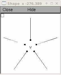
Now display everything:
shape_window = h.PlotShape()
shape_window.exec_menu('Show Diam')
Make a NetStim
Okay, we have our ball-and-stick cells arranged in a ring. Let’s now stimulate a cell and see that it is alive. Instead of stimulating with a current electrode as we did before, let’s assign a virtual synapse so that we get acquainted with driving the cells through synaptic events.
Event-based communication between objects in NEURON takes place via network connection objects call NetCons. Each NetCon has a source and target, where the source is typically a spike threshold detector. When a spike is detected, the NetCon sends a message to a target, usually a synapse on a postsynaptic cell.
A NetStim is a spike generator that can be used as the source in a NetCon, behaving as external input onto the synapse of a target cell. The following code makes a NetStim object that generates one spike at time t=9. The NetCon then adds another ms delay to deliver a synaptic event at time t=10 onto the first cell.
The code below makes a stimulator and attaches it to a synapse object (ExpSyn) that behaves much like an AMPA synapse – it conducts current as a decaying exponential function.
stim = h.NetStim() # Make a new stimulator

# Attach it to a synapse in the middle of the dendrite
# of the first cell in the network. (Named 'syn_' to avoid
# being overwritten with the 'syn' var assigned later.)
syn_ = h.ExpSyn(cells[0].dend(0.5))

stim.number = 1
stim.start = 9
ncstim = h.NetCon(stim, syn_)
ncstim.delay = 1
ncstim.weight[0] = 0.04 # NetCon weight is a vector.
Let’s change the tau to decay by 2 ms.
syn_.tau = 2
We can see syn_’s properties.
print(dir(syn_))
print('tau = {}'.format(syn_.tau))
print('reversal = {}'.format(syn_.e))
Let’s visualize the results of a simulation.
soma_v_vec, dend_v_vec, t_vec = simrun.set_recording_vectors(cells[0])
simrun.simulate()
simrun.show_output(soma_v_vec, dend_v_vec, t_vec)
pyplot.show()

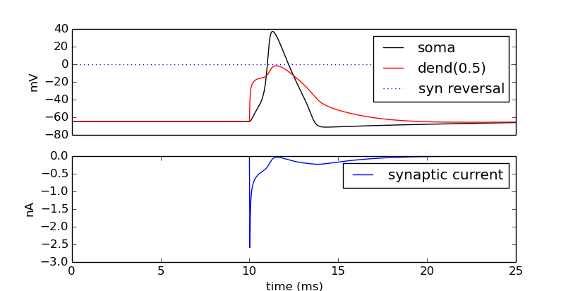
How might we view the synaptic conductance during the simulation?
# Set recording vectors
syn_i_vec = h.Vector()
syn_i_vec.record(syn_._ref_i)

simrun.simulate()

# Draw
fig = pyplot.figure(figsize=(8,4))
ax1 = fig.add_subplot(2,1,1)
soma_plot = ax1.plot(t_vec, soma_v_vec, color='black')
dend_plot = ax1.plot(t_vec, dend_v_vec, color='red')
rev_plot = ax1.plot([t_vec[0], t_vec[-1]], [syn_.e, syn_.e],
        color='blue', linestyle=':')
ax1.legend(soma_plot + dend_plot + rev_plot,
        ['soma', 'dend(0.5)', 'syn reversal'])
ax1.set_ylabel('mV')
ax1.set_xticks([]) # Use ax2's tick labels

ax2 = fig.add_subplot(2,1,2)
syn_plot = ax2.plot(t_vec, syn_i_vec, color='blue')
ax2.legend(syn_plot, ['synaptic current'])
ax2.set_ylabel(h.units('ExpSyn.i'))
ax2.set_xlabel('time (ms)')
pyplot.show()
Try setting the recording vectors to one of the other cells. They should be unresponsive to the stimulus.
Connect the cells
Okay. We have our ball-and-stick cells arranged in a ring, and we’ve attached a stimulus onto the first cell. Next, we need to connect an axon from cell n to a synapse at the middle of the dendrite on cell n + 1. For this model, the particular dynamics of the axons do not need to be explicitly modeled. When the soma fires an action potential, we assume the spike propagates down the axon and induces a synaptic event onto the dendrite of the target cell with some delay. We can therefore connect a spike detector in the soma of the presynaptic cell that triggers a synaptic event in the target cell via a NetCon.
nclist = []
syns = []
for i in range(N):
    src = cells[i]
    tgt = cells[(i + 1) % N]
    syn = h.ExpSyn(tgt.dend(0.5))
    syns.append(syn)
    nc = h.NetCon(src.soma(0.5)._ref_v, syn, sec=src.soma)
    nc.weight[0] = 0.05
    nc.delay = 5
    nclist.append(nc)
Confirm that we get results.
soma_v_vec, dend_v_vec, t_vec = simrun.set_recording_vectors(cells[0])
simrun.simulate(tstop=100)
simrun.show_output(soma_v_vec, dend_v_vec, t_vec)
pyplot.show()
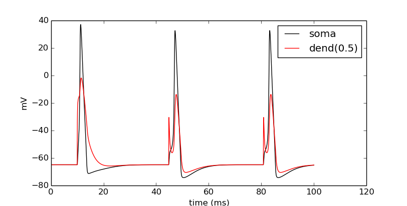
Try this again with a different cell instead of cells[0] (i.e. try cells[1] through cells[N - 1]).
We can see that the network is now active – an initial trigger generates a spike in the first cell, which generates a spike in the second cell, etc., looping on and on. One thing that we did not do was record all of the spike times. Let’s do that with NetCon.record().
spike_times = [h.Vector() for nc in nclist]
for nc, spike_times_vec in zip(nclist, spike_times):
    nc.record(spike_times_vec)

simrun.simulate(tstop=100)
Print out the results.
for i, spike_times_vec in enumerate(spike_times):
    print('cell {}: {}'.format(i, list(spike_times_vec)))
Each line represents one cell and lists all the times it fires: cell 0 fires first, then 1, 2, 3, 4, back to 0, etc.
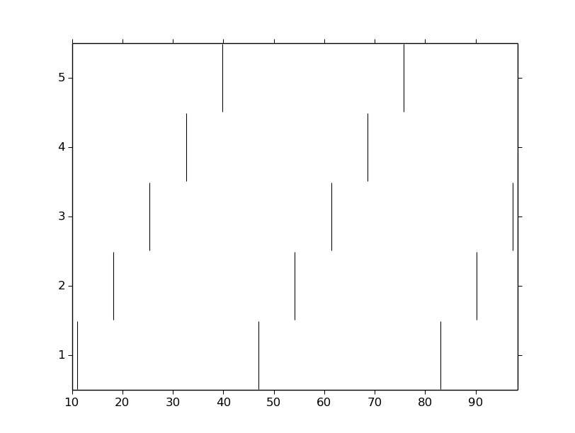
We can also visualize raster plots:
pyplot.figure()
for i, spike_times_vec in enumerate(spike_times):
    pyplot.vlines(spike_times_vec, i + 0.5, i + 1.5)
pyplot.show()
This page has demonstrated various functionality to arrange, connect, and visualize a network and its output. As nice as it may seem, it needs some design work to make it flexible. The next part of the tutorial further organizes the functionality into more classes to make it more easily extended.